This project was completed for Machine Learning I, @ George Washington University, with Lee Eyler, Jacob McKay, and Mikko He. The python code for this project is can be found here.

Background

Apartment hunting is challenging. For the renter, the process of relocating, assessing housing options, and making a long-term decision on a residency can be a tiring and time consuming process. For the landlord or broker, the task of identifying how best to showcase and price a listing can be complex and overwhelming. Companies such as RentHop are trying to simplify the apartment hunting process for everyone involved using a data-driven approach.

The below analysis was completed by our Finance and Economics team while participating in the Two Sigma Connect: Rental Listing Inquiries competition on Kaggle. The competition is focused on accurately predicting the demand for rental properties in the New York City area using data provided by Rent Hop. Two Sigma posed the question: How much interest will a new rental listing on RentHop receive in New York City? To solve this problem, we created a multi-class prediction model that accurately assigns probabilities to the demand level classes for a particular rental listing.

The prediction model is important because it provides a foundation for: 1. Exploring the types of apartment features that are most indicative of demand 2. Matching availability and demand expectations between landlords/brokers and renters 3. Identifying irregular patterns between listing information and demand

Feature Engineering

Renthop provides a comprehensive set of 14 independent attributes that cover many of the key determinants of demand, such as physical location, price, bedroom/bathroom counts, etc.

The dataset did not require extensive cleansing, thus, we focused on the data preprocessing on feature engineering rather than missing data and outliers. This included the creation of 14 variables additional variables through the following engineering:

• Date time (year, month, day, hour, day of week)
• Number of photos (photo_count)
• Price per bathroom and bedroom (price_per_bed; price_per_bedbath)
• If listing has an elevator (Elevator)
• If listing has doorman (Doorman)
• If listing has hardwood floors (Hardwood)
• If listing has laundry (Laundry)
• If listing has a dishwasher (Dishwasher)
• Number of features listed in the “features” column

Feature Importance

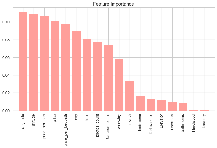
Feature Importance is a method of data analysis that provides a score to see how useful or valuable each feature is. We did this through a random forest classifier; The attribute is used more to make key decisions if it has a higher relative importance.

The Random Forest classifier provided the following results, estimating that about half of the available features are important in regards to decreasing node impurity. The most important predictors are related to location, price, and time.

from sklearn.ensemble import RandomForestClassifier

# select variables; leaving out categorical data for now
X_train_rf_features = X_train[:,[0,1,7,9,12,15,16,17,18,19,20,21,22,23,24,25,26,27]]
y_train_rf_features = y_train
X_test_rf_features = X_test[:,[0,1,7,9,12,15,16,17,18,19,20,21,22,23,24,25,26,27]]
feature_labels = full_df.columns[[1,2,8,10,13,16,17,18,19,20,21,22,23,24,25,26,27,28]]

# set features for RF
forest = RandomForestClassifier(n_estimators=250,
                               random_state=1,
                               n_jobs=-1)
# fit the model
forest.fit(X_train_rf_features,y_train_rf_features)

# obtain feature importances
feat_importance = forest.feature_importances_

# create indices
indices = np.argsort(feat_importance)[::-1]

# print variables and standardized importance score
for f in range(X_train_rf_features.shape[1]):
    print("%2d) %-*s %f" % (f + 1, 30, feature_labels[indices[f]], feat_importance[indices[f]]))

Feature Extraction

Feature extraction is an approach to data compression that projects data onto a new feature space in order to show the most relevant information within the dataset. This is a valuable tool to improve computational efficiency.

The Principal Component Analysis (unsupervised dimensionality reduction) shows that projecting the existing variables onto a smaller subspace can still be highly representative of the original data set. Eight principal components account for ~80% of explained variance.

Principal Component Analysis

from sklearn.decomposition import PCA
pca = PCA(n_components=None)

# only using numeric and categorical data w/ dummy variables
X_train_for_pca = X_train[:,[0,1,7,9,12,15,16,17,18,19,20,21,22,23,24,25,26,27]]

# standardize the data
from sklearn.preprocessing import StandardScaler
stdsc = StandardScaler()
X_train_for_pca_std = stdsc.fit_transform(X_train_for_pca)

# fitting pca to the data
X_train_pca = pca.fit_transform(X_train_for_pca_std)

# obtain feature importances
pca_var_explained = pca.explained_variance_ratio_
feature_labels = full_df.columns[[1,2,8,10,13,16,17,18,19,20,21,22,23,24,25,26,27,28]]

# cumulative sum of explained ration
cumulative_var_explained = np.cumsum(pca_var_explained)

# cumulative distribution function for principle componets
# based on explained variance ratio
sns.set(style="whitegrid")
sns.set_color_codes("pastel")
sns.set_context('talk')

plt.plot(range(X_train_for_pca.shape[1]), cumulative_var_explained)
plt.xlim([-1, X_train_for_pca.shape[1]])
plt.title('Principal Components:  Cumulative Explained Variance Ratio')

Modeling, Evaluation, and Tuning

Three modeling techniques were leveraged:

1. Random Forest
2. K Nearest Neighbors
3. Logistic Regression

Below is a summary of each model, model analysis, and model tuning performed. To assess initial model performance, we used a cross validated accuracy score.

Random Forest

Random Forest is a classification model that is built on an ensemble of decision trees. Decision trees perform the best possible split at each node according to the information gained. This is repeated k number of times, and the predictions are aggregated and assigned class labels based on majority vote.

We chose Random Forest because our network’s input contains several categorical features. Our Random Forest model achieved the following accuracy for predicting level of interest:

[(0.72557776798683371, 0.73174339097955354, 0.73790901397227338)]

These three accuracy scores represent a high/low estimate of accuracy, with the mean minus standard deviation, the mean, and the mean plus one standard deviation, respectively.

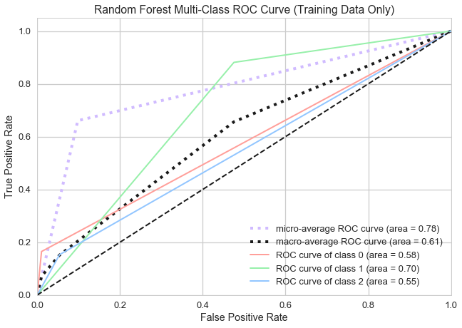
We used a Receiver Operating Characteristic curve (or ROC curve) to plot the true positive rate against the false positive rate for the different possible cutpoints of our model. Our Random Forest model performed best predicting class 1, or “medium” interest listings.

K Nearest Neighbors (KNN)

KNN is a non-parametric classification algorithm that stores all occurrences and classifies new ones on the basis of similarity measurement training.

Using all numeric variables, our KNN model achieved the following accuracy for predicting level of interest:

[(0.66046962839819823, 0.66566638970107761, 0.67086315100395699)]

Using the numeric variables determined by random forest feature selection, our KNN model achieved the following accuracy for predicting level of interest:

[(0.66399494141264304, 0.66850385231130738, 0.67301276320997172)]

The model performed lightly better using the variables determined by random forest feature selection.

Like our Random Forest model, the KNN model performed best predicting class 1, or “medium” interest listings.

Logistic Regression

Logistic Regression is a classification algorithm containing a categorical response variable used for predictive modeling. We chose Logistic Regression because we sought to discover the relationships between our numerous explanatory variables and the categorical response, Level of Interest.

Using all numeric variables, our Logistic Regression model achieved the following accuracy for predicting Level of Interest:

[(0.69152577988828101, 0.69557479886143891, 0.69962381783459682)]

Using the numeric variables determined by random forest feature selection, our Logistic Regression model achieved the following accuracy for predicting level of interest:

[(0.68877017582389244, 0.69138030682828888, 0.69399043783268533)]

The model performed slightly better using all variables.

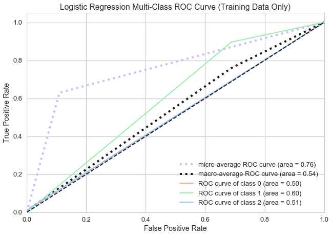
Like both previous models, the Logistic Regression model performed best predicting class 1, or “medium” interest listings.

Performance Optimization

Grid search was chosen for performance optimization. Because it takes a lot of computing power to run, we limited grid search to just one model, Random Forest (as it is the best classifier according to ROC curves).

The grid search provided by Scikit-learn GridSearchCV generates candidates from a “grid” of parameter values. When “fitting” it on a dataset, all the possible combinations of parameter values are evaluated and the best combination is retained. As seen below, the accuracy score was not dramatically improved using grid search.

# initiate random forest for grid search and cross validation
forest = RandomForestClassifier(random_state=1,n_jobs=-1)

# create parameter grid for grid search
crit_param = ['gini','entropy']
tree_param = [300,600]
max_feature_param = [3,6]
gs_param_grid = [{'criterion': crit_param,
               'n_estimators': tree_param,
               'max_features': max_feature_param
              }]
# create grid search object
rf_gridsearch = GridSearchCV(estimator=forest, param_grid=gs_param_grid, scoring='accuracy', cv=5, n_jobs=-1)

# fit grid search model
rf = rf_gridsearch.fit(X_train_rf_features, y_train_rf_features)

rf.best_score_
Out[84]:
0.73097341546441885

rf.best_params_
Out[85]:
{'criterion': 'entropy', 'max_features': 6, 'n_estimators': 600}

Conclusion

Through the utilization of random forest modeling, KNN and Logistic Regression, our team was able to successfully outline the degrees of accuracy between the various predictors of apartment demand. The random forest classifier deemed useful through it’s ability to estimate roughly half of the available features are important in regards to decreasing node impurity. Of those features, those considered the most important in predicting apartment demand are location, price, and time.

From there, our three models enabled us to better understand the high/low estimates of accuracy for predicting apartment demand.

There is further research to be study rental apartment demand using this data which would help improve our accuracy. First, we recommend increasing the domain knowledge of the data, for example, interviews with New York City apartment searchers or real estate professionals. Second, we recommend further feature engineering to improve accuracy. We believe that investing in the Google Maps API will be valuable to provide location data that can be used to target interest level. Finally, we believe that there is room to explore model tuning techniques, beyond grid search, to improve performance and accuracy.